Apple launches Apple Store app in India

The Apple Store app provides customers with the most personalized way to shop for Apple’s innovative lineup of products and services. Learn more >

You can make a difference in the Apple Support Community!

When you sign up with your Apple Account, you can provide valuable feedback to other community members by upvoting helpful replies and User Tips.

Looks like no one’s replied in a while. To start the conversation again, simply ask a new question.

How To Get The Value From Above Cell When Inserting Or Deleting Row In Numbers?

Hello,


I am trying to add from column A (amount) with previous cell in column B, the issue is every time I add/delete/rearrange a row I have to manually re-reference everything. Is there a formula that could always take the value from the direct cell above it without breaking when changes are made?


Posted on Feb 17, 2021 4:27 PM

Reply
Question marked as Top-ranking reply

Posted on Feb 17, 2021 5:35 PM

Try this one, entered in B2 of your table and filled down to the bottom row of column B:


B2: SUM(A$1:A2)


When filled down, the range will expand to include the row containing the new copy of the formula.


Values in column A are all entered fom the keyboard. Valies in column B are all calculated by a copy of the formula above, entered in B2 of Table 1, and filled down to the last row of that tables.


The table on the left is the original. Text below the others tell what changes were made on a copy of the table to its immediate left.


All adjustment of the formulas to fit their new positions, and all addition of formulas to new rows was done automatically by Numbers.


The 'New row 10' was added by clicking the row control button at the bottom of the row reference tabs once.


The new row inserted 'blow' row 4 was inserted by:

Click once on any bell in row 4.

Press option-down arrow.


Regards,

Barry

13 replies
Question marked as Top-ranking reply

Feb 17, 2021 5:35 PM in response to bnajmeddine

Try this one, entered in B2 of your table and filled down to the bottom row of column B:


B2: SUM(A$1:A2)


When filled down, the range will expand to include the row containing the new copy of the formula.


Values in column A are all entered fom the keyboard. Valies in column B are all calculated by a copy of the formula above, entered in B2 of Table 1, and filled down to the last row of that tables.


The table on the left is the original. Text below the others tell what changes were made on a copy of the table to its immediate left.


All adjustment of the formulas to fit their new positions, and all addition of formulas to new rows was done automatically by Numbers.


The 'New row 10' was added by clicking the row control button at the bottom of the row reference tabs once.


The new row inserted 'blow' row 4 was inserted by:

Click once on any bell in row 4.

Press option-down arrow.


Regards,

Barry

Feb 17, 2021 10:49 PM in response to bnajmeddine

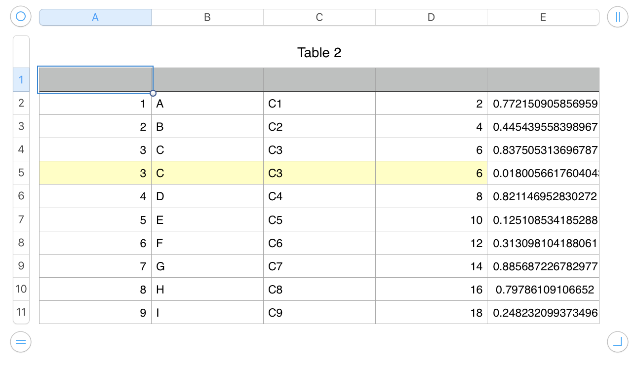
Here's and example using INDEX and a fixed reference to $A$1. The yellow filled row has the formula in all columns except column E.

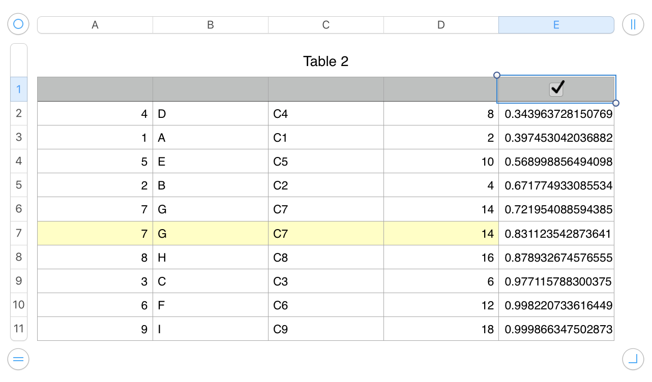
Cells in column E contain RAND() which generates a pseudo random value between 0 and in each cell containg the function whenever there's a change in the table. he change in this case is a click on the checkbox cell in E1, toggling its value between true and false.


The table was sorted after each click on the checkbox (added after the first image was taken), and a screenshot taken if the sort resulted in a different position of the colour filled row.


The formula, shown below the last table copies the value from the cell above by creating a pair of index values pointing to that celll.


Original:

Sorted:
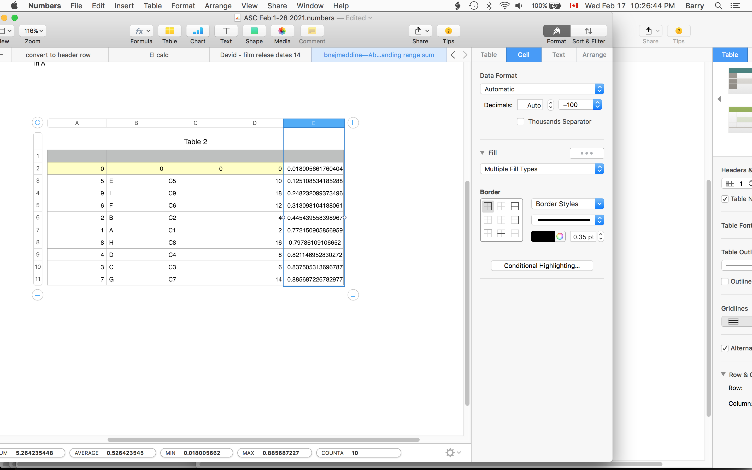
Empty cells (as seen in row 1) return a value of zero.


Third example (note that checkbox has been added in cell E1)
Fourth (and last) example:
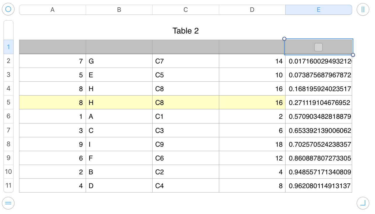
Formula: (copied from cell A5 in table sorted as sorted in Fourth example.)


INDEX($A:$E,ROW()−1,COLUMN())


Regards,

Barry

Feb 18, 2021 9:37 AM in response to Badunit

Thanks again!


Interestingly enough I found the issue it seems that once you've converted the table to categories table it seems to keep the row numbers of the previous table even though the real numbers have changed as a shuffled see examples below.


this is before categorizing by column B, everything seems to work fine with solutions provided and I have also tried with an INDIRECT formula and a CountIF


Here is the row numbers once converted to categories, they are scattered and the wrong cells are referenced.


Any thoughts on how this can be corrected for?


Regards,

Belal

Feb 17, 2021 7:11 PM in response to Barry

Thank you Barry for the detailed explanation. The solution you provided work in all editing situations except for rearranging rows.


If I try to manually rearrange cells or use it in a categories table that is constantly shuffling rows based on other inputs the "sum" formula scatters.


I was trying to use an indirect formula, something like this https://www.extendoffice.com/documents/excel/4385-excel-reference-cell-above.html but I can't seem to make it work in numbers.


Any other ideas would be greatly appreciated

Feb 18, 2021 6:10 AM in response to bnajmeddine

An answer to your question "Is there a formula that could always take the value from the direct cell above it without breaking when changes are made", the OFFSET function can do that, except it cannot because of a bug.


Here is the function. It works perfectly fine if you move rows or delete rows around but NOT if you add new rows. That is the bug, it will give incorrect results until you copy/paste or re-fill the formula into the column or put a new value in column A in that will make the column of formulas recalculate.


B2 =SUM(A2,OFFSET(B2,−1,0))


I used the SUM function vs the + operator so that the formula could be used in B2, where it is picking up the word "total" from the cell above. The + operator will throw an error on text. The SUM function will ignore text.


I thought the OFFSET function was broken when it came to doing this


Feb 18, 2021 6:29 AM in response to Badunit

Sorry for the disjointed post (in particular that last sentence). I recalled the bug after I wrote up how to use the formula and then went back to edit in that problem and didn't proofread my post well enough before submitting it.


I put in a bug report. I don't know if one was submitted the last time this came up, a month or more ago. Hopefully this and the problem with COUNTIF when sorting and a problem with labels on charts will get worked out soon.

Feb 18, 2021 12:06 PM in response to bnajmeddine

I did not try categorizing my test table. What appears to be happening is they are all keeping their original values even though the table got all rearranged/sorted by categorizing it. For example, in the original table in the OFFSET column, the first "A" has a value of 8, the next "A" is 70, etc. The freshly categorized table kept those values in that order. The row numbers on the left of the categorized table do not correspond with the cell references in the formulas. It is like it is in some in-between state.


If you un-categorize then re-categorize (temporarily turn it off then back on in the sidebar), does that give the result you are looking for? If not, explain the result you expect when categorized and we'll try to get it.

Feb 18, 2021 12:13 PM in response to bnajmeddine

The shuffling/sorting of rows is one thing I do not like about categories. When I turn it off I'd like to see my original table in the order it had been. But it appears in your situation the first big issue is, whenever you make a change when categorized, you have to turn it off then back on to get the correct result. You had not mentioned other formulas and their references. Does sorting the table (not categorizing it) also break those references? Maybe that is just a matter of how the cells are being referenced and something can be done.

Feb 18, 2021 2:16 PM in response to bnajmeddine

I seriously did not know you could access subtotals, etc. from the categories. I could swear in the past they were for display only. Don't those links to the subtotals come right back to life when you turn categories back on? They do for me. Maybe we are doing different things?


In your other formulas, you could calculate subtotals with SUMIF or SUMIFS instead of using the category subtotals

How To Get The Value From Above Cell When Inserting Or Deleting Row In Numbers?

Welcome to Apple Support Community
A forum where Apple customers help each other with their products. Get started with your Apple Account.