There are a couple of ways of doing this.
> in my head the formula would be (price*15% if g=hib 10% if g=midt 0% if g=watt)
First off, realize that in Numbers, the IF() statement is based on the model:
=IF(<condition>, <value if true>, <value if false>)
So you could determine the fee rate by checking IF() the vendor = "Hib". If that's true, then assign a fee of 15%
Assuming your table looks something like this:
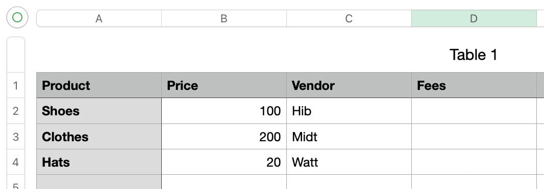
The formula in D2 would be:
=IF(C2="Hib",0.15,0)
That's all well and good for a single vendor. To calculate the others, you evaluate them in the <value if false> part of the formula... so now it starts to look a little gnarly:
=IF(C2="Hib",0.05,IF(C2="Midt",0.1,0))
so now it checks if C2 is "Hib"... if it is we get 0.15, otherwise we run another check to see if C2 is "Midt". Depending on that we get .01 or 0.
Not terrible, and that may be enough for you. However, as you have more vendors, the formula gets more and more unwieldy. And heaven help if you ever need to change the rates.
To that end, there's an arguably better way of doing it - namely via a lookup.
Create a separate, mini table on your sheet (or on another sheet if you don't want to see it) that contains your vendors and their respective fees:
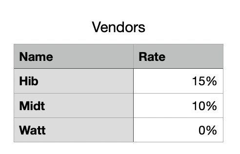
Now on your main sheet, you can perform a LOOKUP() to find the vendor in question and return the appropriate fee rate.
As per the above example, set cell D2 to:
=XLOOKUP(C2,Vendors::Name,Vendors::Rate,0,0,1)
It should look like:
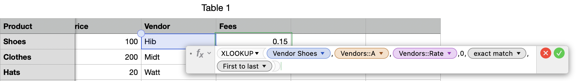
This tells Numbers to take the value in C2 and look it up in the 'Name' column of the 'Vendors' table (make sure your table name matches). For any found result, it returns the corresponding value from the 'Rate' column.
The numbers at the end tell Numbers what to do if the vendor wasn't found (I return 0), and how to search (exact match, top-to-bottom).
The beauty of this is that a) your sheet formulas are much simpler, without nested IF() statements, b) it's trivial to add more vendors over time - just add them to the Vendors table - and c) if the rates change you just need to change them on this sheet and all references will automatically update.