how to LOOKUP in a 2D array

How can I search for a value in one array and output a result in a second array using the same relative position?


for example I there is a calendar month. I want to look up a date and output a value that is in the same relative position a few columns to the right.


what would be a good approach to that?


MacBook Pro 16″, macOS 15.3

Posted on Feb 14, 2025 9:18 AM

Reply
Question marked as Top-ranking reply

Posted on Feb 14, 2025 9:52 AM

That's almost the literal definition of the XLOOKUP() function:


=XLOOKUP(search-value,search-range,return-range,if-not-found,match-type,search-type)


Where search-value is the value to look for,

search-range is the range to search in

return-range is the matching range to return a result from

if-not-found is a value that's returned if search-value is not found

match-type and search-type are fields that tell XLOOKUP how to search (e.g. exact match, first-to-last)


So, given something like:


=XLOOKUP(A2, B, F, "Not Found", exact match, first to last)


this will search column B for the value in A2 using a top-down, exact-match search. If there's a match it will return the corresponding value from column F. If it's not found it will return the string "Not Found"

6 replies
Question marked as Top-ranking reply

Feb 14, 2025 9:52 AM in response to papalapapp

That's almost the literal definition of the XLOOKUP() function:


=XLOOKUP(search-value,search-range,return-range,if-not-found,match-type,search-type)


Where search-value is the value to look for,

search-range is the range to search in

return-range is the matching range to return a result from

if-not-found is a value that's returned if search-value is not found

match-type and search-type are fields that tell XLOOKUP how to search (e.g. exact match, first-to-last)


So, given something like:


=XLOOKUP(A2, B, F, "Not Found", exact match, first to last)


this will search column B for the value in A2 using a top-down, exact-match search. If there's a match it will return the corresponding value from column F. If it's not found it will return the string "Not Found"

Feb 16, 2025 7:34 AM in response to papalapapp

If the dates are in order, one way to do it would be using some math based on the the first date in the array. But I was playing around with how to do this problem in general, where it could be text or something else in the cells, and came up with this idea given below. I feel it is a little sketchy, though, and if you do something slightly different (add an additional column, have two/no header rows, have the "array" in the middle of the table, etc.) you will have to rework the formulas.


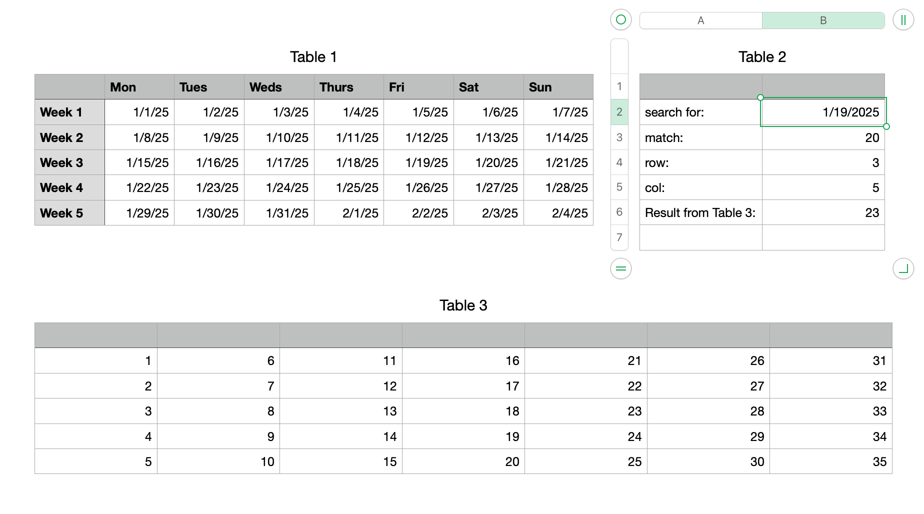
Formulas in Table 2:

B3 =MATCH(B2,UNION.RANGES(FALSE,Table 1::B2:H6,A1),0)

B4 =ROUNDUP((B3−1)÷7,0)

B5 =B3−(B4−1)×7−1

B6 =INDEX(Table 3::A2:G6,B4,B5)

Cell A1 should be empty. It is going to be included in the "array" and you do not want it to be a match by accident.


B3 is the count starting at the first cell in the range, counting up to the last column, moving to the second row of the range, and so on.

B4 and B5 calculate the position.

B6 gets the data from the "different area".


Anyway, I think this works. I'm not 100% clear on UNION.RANGES. It tries to make a 2-D rectangular range from the ranges you give it. If it is not rectangular already it will move rows to the end of the first row until it becomes rectangular. By including one extra cell (A1) in addition to an already rectangular range (B2:H6) I think this will prevent it from making a 2-D array (it is always off by one) so it ends up being one long row, a 1-D array. For some reason, A1 becomes the first cell in the range, regardless of whether I put it first or last in the list.


Feb 14, 2025 3:12 PM in response to papalapapp

I'm not clear on what you are asking. The usual question about searching a 2-D array is about matching something in the top row and matching something in the first column then returning the value at the intersection. An example would be searching for a month name (like "January") in row 1 and a category (like "food") in column A to find how much you spent on food in January. The same formulas can be used to return the "relative position" (the row and the column) of the cell instead of its contents. But I am wondering if you are asking about searching for something within a 2-D array and returning the position of the matching cell. I don't off-hand know of a simple solution to that. One way would be to use MATCH on each row and each column (an n x m array would require n+m individual MATCH formulas) and using additional formulas to determine the intersection. Or it might be able to be done in one formula with the use of UNION.RANGES as long as it is a relatively small array (a small number of rows or columns).


Which of these are you looking to do, or something else?

Feb 15, 2025 11:43 PM in response to Badunit

Thanks for these thoughts. The example of XLOOKUP searches just one column but not multiple rows and columns.


perhaps let me illustrate my case. The area I want to search is 7 columns (mon-sun) and 5 rows or more (weeks). Every cell has the date of that specific day, for example Jan 1 2025.

now I want to look up a specific date - for example Jan 15 2025 - and return the value in a different area at the same relative position.

This thread has been closed by the system or the community team. You may vote for any posts you find helpful, or search the Community for additional answers.

how to LOOKUP in a 2D array

Welcome to Apple Support Community
A forum where Apple customers help each other with their products. Get started with your Apple Account.