Counting events (text entries) in a Numbers table

Mac OS Numbers:


I have created a calendar using a Numbers template.


Into many calendar days I have entered a three letter location. Generally, I use two locations but I would like to be able to add a few more as the need arises.


I want to be able, at any time during the year, to count the number of days spent at either (or any) of the entered locations.


For example, 'how many days were spent at location 'A' in January, or February, or March?' or, how many days were spent at that location during all of those three months?


and then, the same for a second location.


I have tried stumbling through this using 'COUNTIF' but I can’t make it work for my table. Examples I have followed use only two columns.


Can anyone offer me guidance?


Thank you.


MacBook Pro (2021)

Posted on Mar 11, 2025 3:48 PM

Reply
Question marked as Top-ranking reply

Posted on Mar 11, 2025 5:56 PM

5 replies

Mar 11, 2025 4:56 PM in response to ghdghd

A lot of this depends on your layout and table structure. Including how you're using the labels.

For example, is the cell value exactly 'A', or 'B', or 'C'? or are there other notes, annotations, etc.


In either case, there are typically three approaches to this kind of problem.


You've already encountered COUNTIF(), which is a start. If it's not enough, there's also COUNTIFS() which supports multiple conditions.


The next step is filters, which can automatically suppress your table to show only rows with certain values. It may be sufficient to filter on location 'A' and get the data you want (using a footer row on the table, perhaps?).


The ultimate weapon, though, is a pivot table, which is designed to slice and dice a table of data and summarize it in multiple ways.


All are dependent on your table layout, though. If you can give an idea of what it looks like (with dummy data, of course), I'd be happy to dive a little deeper.

Mar 12, 2025 11:18 AM in response to ghdghd

OK, that helps some.. Still not entirely clear, though.


I'm assuming that you want to count how many times NYC appears as well as YVR.


As ever, the devil is in the details. Take Monday the 5th, for example (currently 'NYC').

Is ''NYC" the only thing that would ever appear in that cell?

or might it say something like:


NYC

10 am Meeting with Bob

12pm Lunch with Judy

8:50pm UA123 JFK-LHR


which complicates things a little. Not critically,. but it would be good to understand.


I'm also not sure why your existing formula is referencing cells C8 and E8 - aren't these the day numbers, not the days' agenda/location?


Either way, the formula for the number of 'NYC' in the month (Table 1::B2) would look something like:


=COUNTIF(Calendar::$A$3:$G$13,$A2)


It's simply a COUNTIF() statement, counting all cells in the table.


It's performing a lookup using $A2 as the lookup key, which makes it easy to fill this formula down the column and it will automatically pickup whatever value is in column A as the key (e.g. there's no need to specifically say 'NYC' or 'YVR' in the formula, just have the formula lookup the search value in column A).


That only works great for one month, however a similar indirection can be used for the various months of the year.


Here, I added additional columns, one per month:


And all the cells have the same formula, using a reference to column A for the label, and row 1 for the month.

This relies on naming the tables by month - so instead of one table called 'Calendar', you have one table called 'January', another called 'February', "March", etc. and the formula uses a combination of the header cell and row to work out which values to sum.


Specifically, the formula in cell B2 is:


=COUNTIF(INDIRECT(B$1&"::$A$3:$G$13"),$A2)


Breaking it down, the core is:


=COUNTIF(INDIRECT(B$1&"::$A$3:$G$13"),$A2)


which uses INDIRECT() to find which cells to search, combining the value from B$1 (the header row in this column) to find the month name with the cells range to end up with something like "January::$A$3:$G$13" which is a valid reference that COUNTIF() can use to lookup the search value from $A2. Copy this across the columns and it automatically substitutes the month name taken from the header row to find out where to look.


Once you have this table, it's easy to add any other lookups and functions you want, such as monthly reporting, ranges, etc.


Hope that helps.

Mar 12, 2025 2:28 PM in response to ghdghd

I appreciate the time you are taking to walk through this with me, and your guidance certainly does help.


The answers to your questions:


"Is ''NYC" the only thing that would ever appear in that cell?"


YES. Creating a table like this is new to me and I am keeping things as simple as possible. This table/calendar is specific to this project.


So that you know, and for clarity, I am using this new table to count days in either location, NYC and YVR, only. My concept is to create a calendar that shows how many days were spent in NYC and YVR each month, (each month containing two cells that show that total) and two more cells that show a running total (cumulative) of the number of days spent in NYC and YVR for the year. those two cells will appear once at either the beginning or the end of the year.


Entries will be made 'as they happen', if you know what I mean.


"aren’t these the day numbers, not the days' agenda/location?"


YES, they are. I highlighted those by mistake. And, I kept day numbers in separate cells so as not to confuse either myself or 'Numbers'.


I might be able to work through that which you wrote following that question, and I hope I can. I will say that the table you introduced show results much like that for which I am aiming.


Further, (for the moment) I will say that your formulas do not look like mine, as mine show no '$' entries. About that, I do not know what I do not know.

Mar 13, 2025 10:56 AM in response to ghdghd

> Further, (for the moment) I will say that your formulas do not look like mine, as mine show no '$' entries. About that, I do not know what I do not know.


Ahh, that's how Numbers shows absolute vs. relative addresses. Let me explain...


'Normal' cell references use relative addresses, so they 'float' as you move around the spreadsheet - they are relative to the cell the formula is in.

Absolute cell references (that use the $) are absolute, and always refer to the same row and/or column.


For a single cell, it makes no difference.

If you set cell B2 to either:


=A2 (relative)


or


=$A$2 (absolute)


you get the exact same result in B2.


The difference comes when you use Fill to expand your table.


If you take cell B2 and fill down, all the cell references will update to maintain the same relative offset. Since B2 references A2 (one column to the left), the cells as they fill down will continue to reference 'one column to the left':


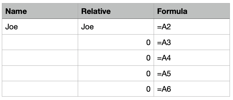
(here, column C is using FORMULATEXT() to show the formula in the adjacent B column)


Now you can see the cell B3 is referencing A3 (relative: one column to the left), and that's empty. Likewise for the rest of the column.


Now, this may be what you want, but sometimes you want the cell to always reference cell A2 and not update as you fill down. You could fill down, then go through and update all the references, but absolute references take care of that.


To set absolute references, click on the disclosure triangle alongside the cell reference in the formula editor. You'll see a little pop-up with options to 'Preserve Row' and 'Preserve Column':


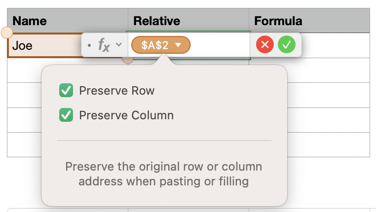
You can choose either row or column, or both, depending on what you want. In this case, I ALWAYS want to reference cell A2, so I preserve both:


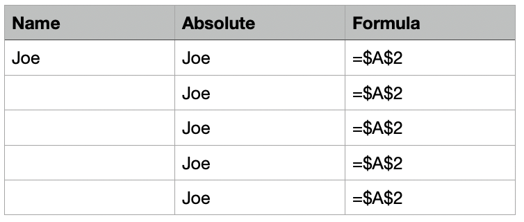
Now as I fill B2 down the column, the cell references remain anchored to $A$2:


That's why I used Absolute references in your summary table:


=COUNTIF(INDIRECT(B$1&"::$A$3:$G$13"),$A2)


This formula added in B2 works great, for B2 but would break if I fill across...


For example, I use $A2 to extract the location name to search for. If this reference were simple A2, then it would update as it moved across the table and break the model.

Similarly, when I look for the month name from the table header, I always want to refer to row 1, not simply "one row above", hence the B$1... as I fill the table, the column B will update, but the $1 will remain fixed.


(Technically, I didn't have to add absolute references in the "::$A$3:$G$13" where "::A3:G13" would have sufficed, since this is just a text string at this point, and not actually a reference, so Numbers wouldn't update it and it would stay the same, but it's a good habit to get into when dealing with specific cells/locations on the table.)


An even clearer example would if you have a table for rates - hourly pay, tax rates, etc. and a separate cost sheet. Let's say I have a Rates table:
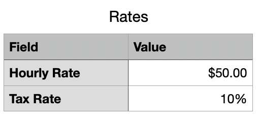


and a cost sheet:


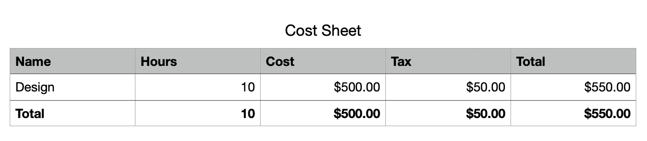
If the cost sheet uses relative addressing, then the Design Cost will correctly reference Rates::B2

But as I add additional costs in additional rows, the relative addressing app update to the same relative offset, and go haywire:


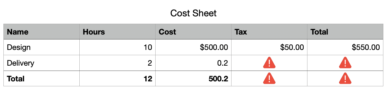
Now, delivery cost is trying to reference Rates::C2 and the tax is broken, trying to reference a non-existent tax cell.


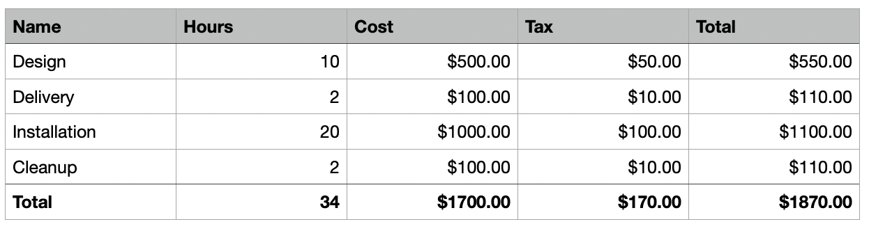
Instead, these formulas should use absolute addressing, so they always go to the rate and tax cells:


By changing cell C2 to:


=B2 * Rates::$B$2


it always references the hourly rate cell and the rest of the table just works:


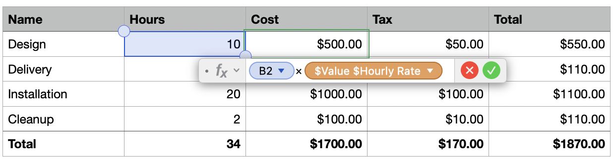
The final note is that Numbers can optionally show column references such as B2, or can substitute labels based on the row and column headers. This is set in Numbers -> Settings -> Use header names as labels.


This setting could change the display from "Rates:$B$2" to "$Value $Hourly Rate" (based on the header columns in the Rates table). The principle of absolute vs. relative addressing still stands, though.


Personally, I flip between using header names and direct references. Can't quite decide which I prefer more.


This thread has been closed by the system or the community team. You may vote for any posts you find helpful, or search the Community for additional answers.

Counting events (text entries) in a Numbers table

Welcome to Apple Support Community
A forum where Apple customers help each other with their products. Get started with your Apple Account.