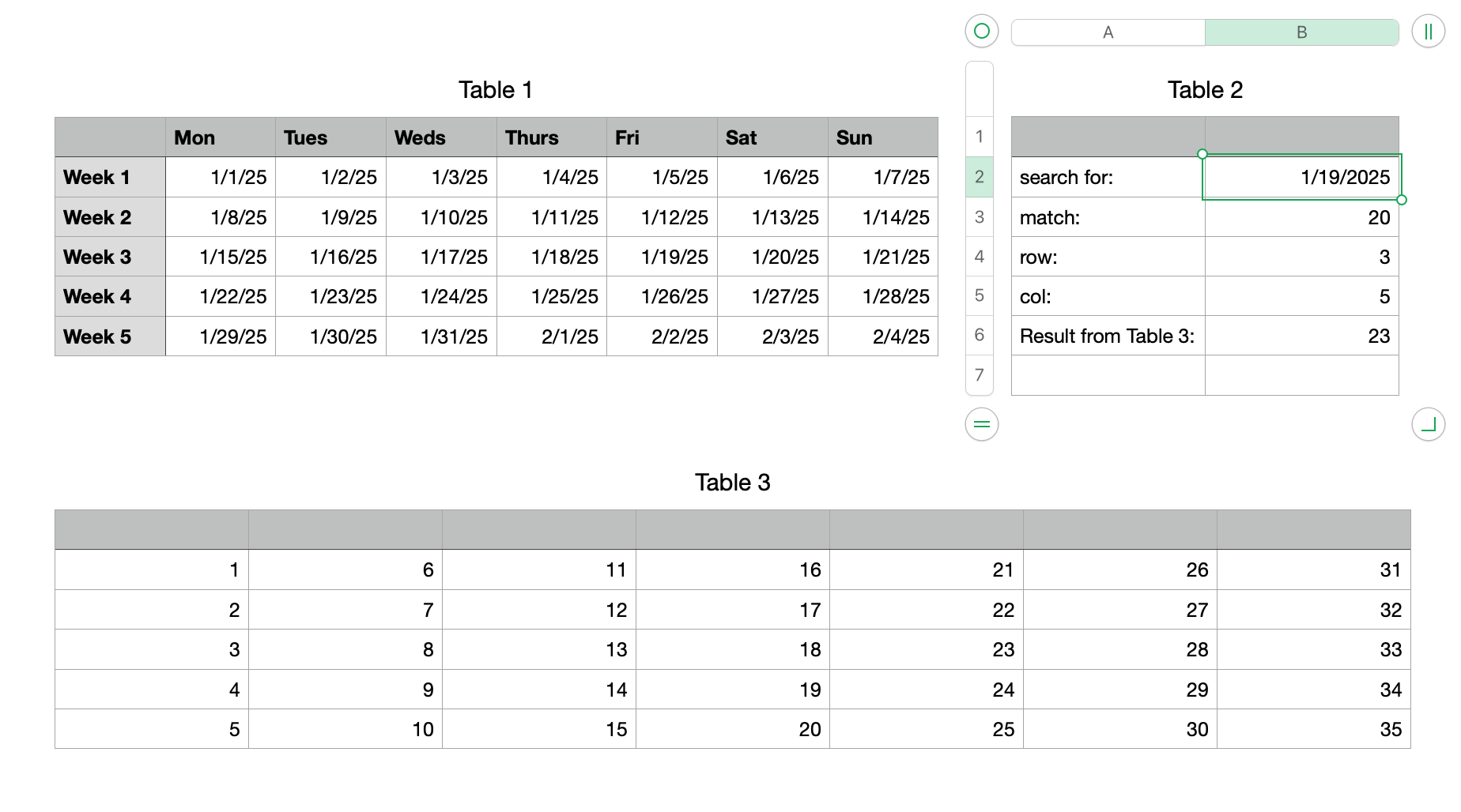
If the dates are in order, one way to do it would be using some math based on the the first date in the array. But I was playing around with how to do this problem in general, where it could be text or something else in the cells, and came up with this idea given below. I feel it is a little sketchy, though, and if you do something slightly different (add an additional column, have two/no header rows, have the "array" in the middle of the table, etc.) you will have to rework the formulas.

Formulas in Table 2:
B3 =MATCH(B2,UNION.RANGES(FALSE,Table 1::B2:H6,A1),0)
B4 =ROUNDUP((B3−1)÷7,0)
B5 =B3−(B4−1)×7−1
B6 =INDEX(Table 3::A2:G6,B4,B5)
Cell A1 should be empty. It is going to be included in the "array" and you do not want it to be a match by accident.
B3 is the count starting at the first cell in the range, counting up to the last column, moving to the second row of the range, and so on.
B4 and B5 calculate the position.
B6 gets the data from the "different area".
Anyway, I think this works. I'm not 100% clear on UNION.RANGES. It tries to make a 2-D rectangular range from the ranges you give it. If it is not rectangular already it will move rows to the end of the first row until it becomes rectangular. By including one extra cell (A1) in addition to an already rectangular range (B2:H6) I think this will prevent it from making a 2-D array (it is always off by one) so it ends up being one long row, a 1-D array. For some reason, A1 becomes the first cell in the range, regardless of whether I put it first or last in the list.